Ta-belle
Sto iniziando a studiare due pacchetti di R che mi sembrano interessanti
Il primo promette di
- To facilitate complex data transformation, exploration and computing tasks in R.
- To help make R code fast, flexible, parsimonious and programmer friendly.
Il secondo dovrebbe essere uno strumento più moderno e flessibile per generare tavole (o tabelle)
With the gt package, anyone can make wonderful-looking tables using the R programming language. The gt philosophy: we can construct a wide variety of useful tables with a cohesive set of table parts. These include the table header, the stub, the column labels and spanner column labels, the table body, and the table footer.
Per puro gioco potrei riscrivere le righe precedenti così Table 1.
| pacchetto | scopo |
|---|---|
collapse |
|
gt | With the gt package, anyone can make wonderful-looking tables using the R programming language. The gt philosophy: we can construct a wide variety of useful tables with a cohesive set of table parts. These include the table header, the stub, the column labels and spanner column labels, the table body, and the table footer. |
Table 1: Pacchetti
Da notare che i pacchetti appartengono, per così dire, a due universi paralleli: fastverse e tidyverse, ma interagiscono benissimo.
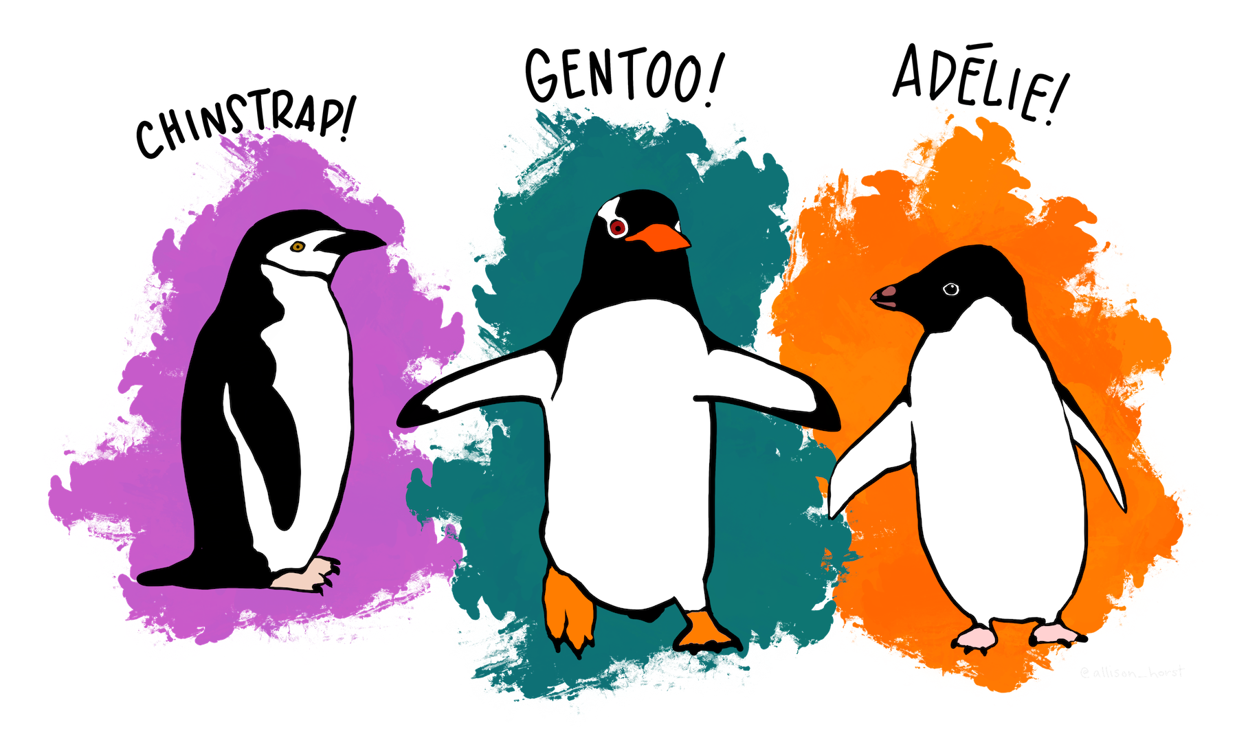
Ora un esempio più corposo usando come dataset penguins contenuto nel pacchetto palmerpenguins. I dati riguardano tre specie diverse di pinguini e sono stati raccolti nella Palmer Station da Kristen Gorman.1 Table 2
Code
su <- collapse::qsu(penguins, by = ~ species + island, cols = 3:6)
sa <- base::aperm(su, c(3L, 2L, 1L))
sa <- as.data.frame(sa)
collapse::setrename(sa, Variable = "Species+Island", Group = Measures)
Il codice crea un qsu (quick summary) del dataset, già eseguendo anche un raggruppamento per specie e isola di origine. Con il comando aperm si permuta il risultato di qsu in modo tale da rendere più semplice la creazione della tabella finale. Con setrename si modificano i nomi di default delle colonne.
A questo punto si può programmare la tabella nella quale verranno esposti i dati.
Code
pi <- sa |> gt() |>
  tab_header(title = md("**I pinguini delle Palmer**"),
             subtitle = "Specie, habitat e caratteri fisici") |>
          tab_row_group(
                        label = "Adelie",
                        rows = 1:12) |>
          tab_row_group(
                        label = "Chinstrap",
                        rows = 13:16) |>
          tab_row_group(
                        label = "Gentoo",
                        rows = 17:20) |>
tab_style(
          style = cell_fill(color = "lightyellow"),
          locations = cells_row_groups(groups = 1)
          ) |>
tab_style(
          style = cell_fill(color = "lightgreen"),
          locations = cells_row_groups(groups = 2)
          )  |>
tab_style(
          style = cell_fill(color = "lightblue"),
          locations = cells_row_groups(groups = 3)
) |>
data_color(
           columns = c(1),
           palette = "viridis"
             )
pi |> tab_options(quarto.disable_processing = TRUE)
| I pinguini delle Palmer | ||||||
| Specie, habitat e caratteri fisici | ||||||
| Species+Island | Measures | N | Mean | SD | Min | Max |
|---|---|---|---|---|---|---|
| Gentoo | ||||||
| Gentoo.Biscoe | bill_length_mm | 123 | 47.50488 | 3.0818574 | 40.9 | 59.6 |
| Gentoo.Biscoe | bill_depth_mm | 123 | 14.98211 | 0.9812198 | 13.1 | 17.3 |
| Gentoo.Biscoe | flipper_length_mm | 123 | 217.18699 | 6.4849758 | 203.0 | 231.0 |
| Gentoo.Biscoe | body_mass_g | 123 | 5076.01626 | 504.1162367 | 3950.0 | 6300.0 |
| Chinstrap | ||||||
| Chinstrap.Dream | bill_length_mm | 68 | 48.83382 | 3.3392559 | 40.9 | 58.0 |
| Chinstrap.Dream | bill_depth_mm | 68 | 18.42059 | 1.1353951 | 16.4 | 20.8 |
| Chinstrap.Dream | flipper_length_mm | 68 | 195.82353 | 7.1318943 | 178.0 | 212.0 |
| Chinstrap.Dream | body_mass_g | 68 | 3733.08824 | 384.3350814 | 2700.0 | 4800.0 |
| Adelie | ||||||
| Adelie.Biscoe | bill_length_mm | 44 | 38.97500 | 2.4809155 | 34.5 | 45.6 |
| Adelie.Biscoe | bill_depth_mm | 44 | 18.37045 | 1.1888199 | 16.0 | 21.1 |
| Adelie.Biscoe | flipper_length_mm | 44 | 188.79545 | 6.7292473 | 172.0 | 203.0 |
| Adelie.Biscoe | body_mass_g | 44 | 3709.65909 | 487.7337218 | 2850.0 | 4775.0 |
| Adelie.Dream | bill_length_mm | 56 | 38.50179 | 2.4653594 | 32.1 | 44.1 |
| Adelie.Dream | bill_depth_mm | 56 | 18.25179 | 1.1336171 | 15.5 | 21.2 |
| Adelie.Dream | flipper_length_mm | 56 | 189.73214 | 6.5850825 | 178.0 | 208.0 |
| Adelie.Dream | body_mass_g | 56 | 3688.39286 | 455.1464371 | 2900.0 | 4650.0 |
| Adelie.Torgersen | bill_length_mm | 51 | 38.95098 | 3.0253180 | 33.5 | 46.0 |
| Adelie.Torgersen | bill_depth_mm | 51 | 18.42941 | 1.3394468 | 15.9 | 21.5 |
| Adelie.Torgersen | flipper_length_mm | 51 | 191.19608 | 6.2322375 | 176.0 | 210.0 |
| Adelie.Torgersen | body_mass_g | 51 | 3706.37255 | 445.1079402 | 2900.0 | 4700.0 |
Table 2: Occhiata rapida
Come inizio non c’è male, magari ho esagerato con i colori, ma li ho usati solo per capire la sintassi. Il concetto è molto simile a quello di ggplot2 in cui si aggiungono strati su strati, d’altronde sempre dalla stessa fucina escono.
Con collapse potremmo anche vedere i dati sotto un altro aspetto, ponendo, per esempio, l’accento sulle caratteristiche fisiche. Table 3
Code
i <- collapse::qsu(penguins, by = ~ island + species, cols= 3:6, array = FALSE)
qw <- unlist2d(i, idcols = c("Variable"), row.names = "Island & Species") |>
  gt() |>
    tab_header(title = md("**I pinguini delle Palmer**"),
             subtitle = "Misure dei caratteri fisici") |>
          data_color(
                     columns = c(1),
                     palette = "viridis"
)
qw |> tab_options(quarto.disable_processing = TRUE)
| I pinguini delle Palmer | ||||||
| Misure dei caratteri fisici | ||||||
| Variable | Island & Species | N | Mean | SD | Min | Max |
|---|---|---|---|---|---|---|
| bill_length_mm | Biscoe.Adelie | 44 | 38.97500 | 2.4809155 | 34.5 | 45.6 |
| bill_length_mm | Biscoe.Gentoo | 123 | 47.50488 | 3.0818574 | 40.9 | 59.6 |
| bill_length_mm | Dream.Adelie | 56 | 38.50179 | 2.4653594 | 32.1 | 44.1 |
| bill_length_mm | Dream.Chinstrap | 68 | 48.83382 | 3.3392559 | 40.9 | 58.0 |
| bill_length_mm | Torgersen.Adelie | 51 | 38.95098 | 3.0253180 | 33.5 | 46.0 |
| bill_depth_mm | Biscoe.Adelie | 44 | 18.37045 | 1.1888199 | 16.0 | 21.1 |
| bill_depth_mm | Biscoe.Gentoo | 123 | 14.98211 | 0.9812198 | 13.1 | 17.3 |
| bill_depth_mm | Dream.Adelie | 56 | 18.25179 | 1.1336171 | 15.5 | 21.2 |
| bill_depth_mm | Dream.Chinstrap | 68 | 18.42059 | 1.1353951 | 16.4 | 20.8 |
| bill_depth_mm | Torgersen.Adelie | 51 | 18.42941 | 1.3394468 | 15.9 | 21.5 |
| flipper_length_mm | Biscoe.Adelie | 44 | 188.79545 | 6.7292473 | 172.0 | 203.0 |
| flipper_length_mm | Biscoe.Gentoo | 123 | 217.18699 | 6.4849758 | 203.0 | 231.0 |
| flipper_length_mm | Dream.Adelie | 56 | 189.73214 | 6.5850825 | 178.0 | 208.0 |
| flipper_length_mm | Dream.Chinstrap | 68 | 195.82353 | 7.1318943 | 178.0 | 212.0 |
| flipper_length_mm | Torgersen.Adelie | 51 | 191.19608 | 6.2322375 | 176.0 | 210.0 |
| body_mass_g | Biscoe.Adelie | 44 | 3709.65909 | 487.7337218 | 2850.0 | 4775.0 |
| body_mass_g | Biscoe.Gentoo | 123 | 5076.01626 | 504.1162367 | 3950.0 | 6300.0 |
| body_mass_g | Dream.Adelie | 56 | 3688.39286 | 455.1464371 | 2900.0 | 4650.0 |
| body_mass_g | Dream.Chinstrap | 68 | 3733.08824 | 384.3350814 | 2700.0 | 4800.0 |
| body_mass_g | Torgersen.Adelie | 51 | 3706.37255 | 445.1079402 | 2900.0 | 4700.0 |
Table 3: Caratteristiche fisiche
Ancora un esempio Table 4.
Code
s <- collapse::qsu(penguins, pid = ~ species, cols = c(3:6), higher = TRUE)
s <- base::aperm(s, c(3L, 2L, 1L))
s <- as.data.frame(s)
collapse::setrename(s, Group = "Caratteri misurati")
dsa <- s |> gt() |>
    tab_header(title = md("**I pinguini delle Palmer**"),
  subtitle = "Caratteri misurati") |>
          data_color(
                     columns = c(1),
                     palette = "viridis"
) |>
tab_footnote(footnote = "Overall è riferito a tutte le osservazioni",
             locations = cells_body(
                                    columns = Trans,
                                    rows = 1
             )
             ) |>
tab_footnote(footnote = "Between-species (i.e. species averaged)",
             locations = cells_body(
                                    columns = Trans,
                                    rows = 2
             )
             ) |>
tab_footnote(footnote = "Within-species (i.e. species-demeaned)",
             locations = cells_body(
                                    columns = Trans,
                                    rows = 3
             )
             )
dsa |> tab_options(quarto.disable_processing = TRUE)
| I pinguini delle Palmer | ||||||||
| Caratteri misurati | ||||||||
| Caratteri misurati | Trans | N/T | Mean | SD | Min | Max | Skew | Kurt |
|---|---|---|---|---|---|---|---|---|
| bill_length_mm | Overall1 | 342 | 43.92193 | 5.459584 | 32.10000 | 59.60000 | 0.05288481 | 2.119235 |
| bill_length_mm | Between2 | 3 | 45.04336 | 5.454989 | 38.79139 | 48.83382 | -0.66018641 | 1.500000 |
| bill_length_mm | Within3 | 114 | 43.92193 | 2.951161 | 35.98811 | 56.01705 | 0.28796688 | 3.530494 |
| bill_depth_mm | Overall | 342 | 17.15117 | 1.974793 | 13.10000 | 21.50000 | -0.14283463 | 2.088845 |
| bill_depth_mm | Between | 3 | 17.24969 | 1.964126 | 14.98211 | 18.42059 | -0.70597072 | 1.500000 |
| bill_depth_mm | Within | 114 | 17.15117 | 1.117532 | 14.30481 | 20.30481 | 0.25892215 | 2.727361 |
| flipper_length_mm | Overall | 342 | 200.91520 | 14.061714 | 172.00000 | 231.00000 | 0.34416383 | 2.012566 |
| flipper_length_mm | Between | 3 | 200.98805 | 14.332413 | 189.95364 | 217.18699 | 0.57602992 | 1.500000 |
| flipper_length_mm | Within | 114 | 200.91520 | 6.622023 | 182.96156 | 220.96156 | 0.16501150 | 2.925426 |
| body_mass_g | Overall | 342 | 4201.75439 | 801.954536 | 2700.00000 | 6300.00000 | 0.46826396 | 2.273757 |
| body_mass_g | Between | 3 | 4169.92225 | 784.867905 | 3700.66225 | 5076.01626 | 0.70574924 | 1.500000 |
| body_mass_g | Within | 114 | 4201.75439 | 460.916730 | 3075.73813 | 5425.73813 | 0.18165543 | 2.507951 |
| 1 Overall è riferito a tutte le osservazioni | ||||||||
| 2 Between-species (i.e. species averaged) | ||||||||
| 3 Within-species (i.e. species-demeaned) | ||||||||
Table 4: Variabilità dei caratteri fisici
Spero che queste poche note facciano incuriosire qualcuno.